Waves Teaching Guide
Conceptual Foundations
Generation of mechanical waves
A mechanical wave is a vibration propagating through a medium. Requirements: a source + a medium. The particles do not travel with the wave; they only vibrate about their equilibrium positions.
Basic relations
- Wave speed : set by the medium
- Frequency : set by the source
- Wavelength : set by both together
Standing-wave condition (string fixed at both ends)
Interference
- Constructive:
- Destructive:
Diffraction
Condition for pronounced diffraction: slit width .
Using the Builder
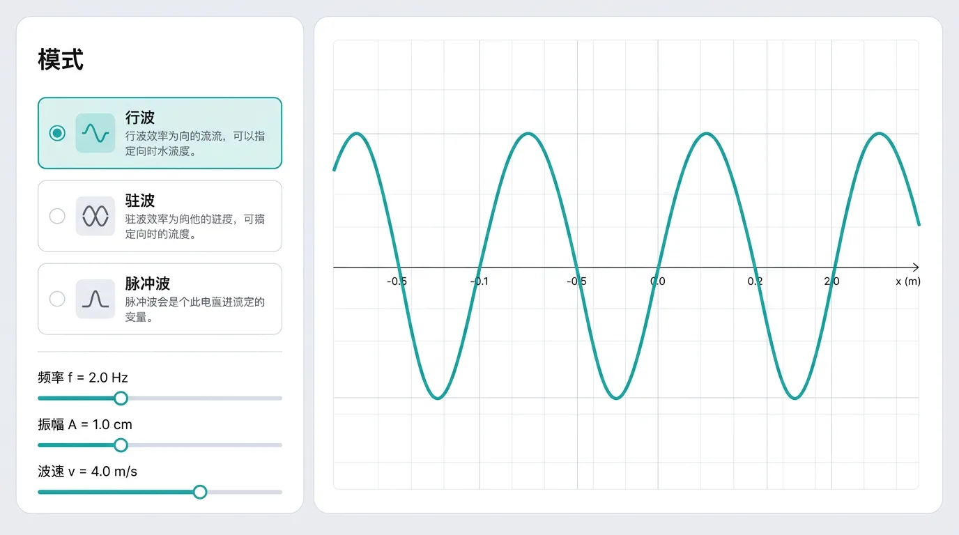
Open the wave builder (nav bar → Builder → Waves). There are two modes:
- 2-D wave field: a top-down water-ripple simulation; observe interference and diffraction patterns
- 1-D wave on a string: transverse waves on a one-dimensional string; observe standing waves, harmonics and reflection
Gestures
| Operation | How |
|---|---|
| Select a source / probe / end | Click the object on the canvas (its properties expand on the left) |
| Move position | Hold and drag |
| Change parameters quickly | Double-click a source, probe or string end to pop up an inline parameter box |
| Getting started | The "Official scenes" dropdown at the top left loads ready-made scenes such as double-slit interference and standing waves |
Detailed Entity Reference
Components of the 2-D wave field mode
Point source (source)
A point source that sends out circular waves in all directions.
| Parameter | Symbol | Unit | Range | Default | Notes |
|---|---|---|---|---|---|
| Amplitude | amplitude | m | 0.01–5 | 1 | The strength of the wave |
| Frequency | frequency | Hz | 0.1–20 | 2.5 | Sets the wavelength |
Use cases:
- Single source: watch circular waves spread outward
- Two sources (same frequency): observe interference fringes
- Several sources: complex interference patterns
Demo notes:
- Two sources must have the same frequency to produce a stable interference pattern
- Different frequencies → beats (the fringes are not stable)
- Dragging a source changes the interference pattern in real time
Obstacle / barrier (barrier)
An obstacle that blocks the wave's progress. It can form slits.
| Parameter | Symbol | Unit | Range | Default | Notes |
|---|---|---|---|---|---|
| Region | region | — | rectangle | — | The barrier's position and size (drag it on the canvas to adjust) |
Building a slit: place two barriers with a gap between them. The slit width is the distance between the two barriers.
Use cases:
- Single-slit diffraction: leave a gap between two barriers
- Double-slit interference: three barriers form two slits
- Bending: the wave curls round the edge of a barrier
Demo notes: with slit width diffraction is weak (the wave passes nearly straight through); with diffraction is most pronounced.
Wave-speed region (region)
Sets a different wave speed inside a rectangular region.
| Parameter | Symbol | Unit | Range | Default | Notes |
|---|---|---|---|---|---|
| Wave speed | speed | m/s | 0.1–5 | 0.5 | Wave speed inside the region, overriding the global default wave speed (priority: region > global) |
Priority: wave speed is defined in 2 places: the global default wave speed and the speed of each wave-speed region. Inside a region the wave travels at the region's value; anywhere no wave-speed region covers it travels at the global default. When several wave-speed regions overlap, the later declaration wins.
Use case: model a wave going from deep water into shallow water (wave speed drops → wavelength shortens → refraction).
Probe (probe2d)
Records how the vibration of one point changes with time (a u-t vibration graph).
| Parameter | Symbol | Unit | Range | Default | Notes |
|---|---|---|---|---|---|
| Position | position | m | canvas range | — | The probe's coordinates (drag it on the canvas to adjust) |
| Observer velocity | velocity | m/s | — | 0 | Advanced: a moving observer produces a Doppler effect |
Use case: place it in regions of constructive/destructive interference and compare the amplitudes. At a node the amplitude is zero.
Boundary (boundary, scene level)
What happens when the wave reaches the canvas edge (default "Absorbing"):
- Absorbing: the wave leaves the boundary without reflecting, modelling open space (use this for interference/diffraction experiments)
- Reflecting wall: a fixed wall; reflection inverts phase (a crest comes back as a trough)
- Free end: reflection in phase (a crest comes back still a crest)
Components of the 1-D wave-on-a-string mode
Sinusoidal driver (sine)
Applies a continuous sinusoidal drive at one point of the string.
| Parameter | Symbol | Unit | Range | Default | Notes |
|---|---|---|---|---|---|
| Position | position | m | 0–10 | 0.2 | The driver's position along the string |
| Amplitude | amplitude | m | 0.01–5 | 0.2 | The driving amplitude |
| Frequency | frequency | Hz | 0.1–20 | 0.125 | The driving frequency |
Use case: produces a continuous travelling wave; when the frequency satisfies a standing wave forms.
Demo notes:
- When the frequency fails the standing-wave condition, the string shows complicated beats (the amplitude grows and shrinks)
- That is itself a valuable observation - it shows that only certain frequencies resonate
Pulse wave (pulse)
Applies a single pulse at one point of the string.
| Parameter | Symbol | Unit | Range | Default | Notes |
|---|---|---|---|---|---|
| Position | position | m | 0–10 | 1.4 | The pulse's starting position |
| Amplitude | amplitude | m | 0.01–5 | 1 | The pulse's height |
| Pulse width | width | m | 0.05–2 | 0.25 | The narrower the pulse, the broader its spectrum |
Use case: watch a single wave packet travel and reflect. Reflection at a fixed end inverts the pulse; reflection at a free end does not.
Standing-wave mode (mode)
Sets the string straight to the initial state of one standing-wave mode (skipping the transient).
| Parameter | Symbol | Unit | Range | Default | Notes |
|---|---|---|---|---|---|
| Harmonic number n | mode | — | 1–10 | 1 | : the number of antinodes |
| Amplitude | amplitude | m | 0.01–5 | 1 | The maximum amplitude at the antinodes |
Use case: observe the shape of the -th standing-wave mode directly, with no waiting for the transient to build up.
Demo suggestions:
- : one antinode, two nodes (the ends)
- : two antinodes, three nodes
- : three antinodes, four nodes
- Check: the spacing of adjacent nodes =
Wave-speed segment (segment)
Sets a different wave speed on one section of the string.
| Parameter | Symbol | Unit | Range | Default | Notes |
|---|---|---|---|---|---|
| Start point | from | m | 0–10 | 2 | Where the segment starts |
| End point | to | m | 0–10 | 4 | Where the segment ends |
| Wave speed | speed | m/s | 0.1–5 | 0.5 | The wave speed on this segment, overriding the whole-string speed (priority: segment > whole string) |
Priority: wave speed is defined in 2 places: the whole-string speed and the speed of each wave-speed segment. Inside a segment the wave travels at the segment's value; outside all segments it travels at the whole-string speed. When several wave-speed segments overlap, the later declaration wins.
Use case: a wave passing from one medium into another (a thick string → a thin string, say); observe transmission and reflection.
Physics: different wave speed → different wavelength (the frequency is unchanged); at the interface the wave partly reflects and partly transmits.
Probe x (probe1d)
Records the displacement-time curve of one point on the string.
| Parameter | Symbol | Unit | Range | Default | Notes |
|---|---|---|---|---|---|
| Position | position | m | 0–10 | 2 | The probe's position on the string |
Use cases:
- At an antinode: maximum amplitude
- At a node: zero amplitude
- Two probes apart: the curves are in antiphase
- Read the period off the - curve
Using the Lab
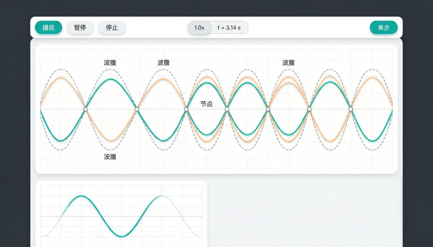
Click "Run it" to enter the lab:
- Play/Pause: watch the wave propagate and superpose
- Speed: 0.25× / 0.5× / 1× / 2× (use slow playback for high-frequency waves)
- Step forward: frame-by-frame stepping; good for judging the direction in which the particles move
- Render modes:
- Waveform rendering: the shape of the string / 2-D colour map (red = crest, blue = trough)
- Particle mode: shows the vibration direction of each particle (proves the particles do not migrate)
- Components (1-D): the incident wave + the reflected wave + the resultant wave shown separately
- Probe curve: the - graph on the right
- Parameter scan: sweep the driving frequency to find the resonance peaks
Common Problems and Cautions
- Standing waves do not travel: normal behaviour. Switch to "Components" to see the incident wave and the reflected wave each in motion.
- Frequency mismatch: unless holds, no stable standing wave forms and beats appear.
- A probe reads zero: it may sit on a node. Move it half a wavelength and you will see maximum vibration.
- Diffraction is weak: with slit width the wave passes almost straight through. Narrow the slit or increase the wavelength (lower the frequency).
- Particles do not migrate: use particle mode to observe - each particle only vibrates up and down; it does not advance with the wave.
- The 2-D wave field stutters: lower the playback speed or shrink the region.
Teaching Suggestions
- Wave-speed equation: fix the wave speed, change the frequency, measure the wavelength, verify that stays unchanged.
- Standing waves: use standing-wave mode to set directly, count the nodes and antinodes, verify .
- Resonance scan: parameter-scan the driving frequency; amplitude peaks appear at .
- Interference: two sources at the same frequency; observe the constructive/destructive fringes and verify the path-difference condition.
- Diffraction: vary the slit width; compare the effects for and .
- Reflection: send a pulse at a fixed end (inverted) and at a free end (not inverted).
Related Experiments
- Transverse waves and standing waves on a string: verify
- Interference of waves: two-source interference fringes
- Single-slit diffraction: the relation between slit width and wavelength
- Doppler effect: move the source and observe wavelengths being compressed/stretched
- Reflection and transmission of waves: behaviour at a boundary between different wave speeds